Reading from file

One of the most common situations is that you want to read your data from a file. In an ideal world the file will be perfectly formatted and will be trivial to import into pandas but since this is so often not the case, pandas provides a number of features to make your life easier.

Full information on reading and writing files is available in the pandas manual on IO tools but first it’s worth noting the common formats that pandas can work with: - Comma separated tables (or tab-separated or space-separated etc.) - Excel spreadsheets - HDF5 files - SQL databases

For this course we will focus on plain-text CSV files as they are perhaps the most common format. It’s also common to be provided with data in an Excel format and Pandas provides all the tools you need to extract the data out of Excel and analyse it in Python.

Reading our first file

You can get access to Pandas by importing the pandas module. By convention, it is imported as pd:

import pandas as pd

We can use the pandas function read_csv() to read a file and convert it to a DataFrame. Full documentation for this function can be found here.

The first argument to the function is called filepath_or_buffer, the documentation for which begins:

Any valid string path is acceptable. The string could be a URL…

This means that we can take a URL and pass it directly (or via a variable) to the function. For example, here is a file with rainfall data:

rain = pd.read_csv("https://bristol-training.github.io/introduction-to-data-analysis-in-python/data/rain.csv")

If this doesn’t work for you…

We have seen in some instances that reading from a URL triggers an error message like

URLError: <urlopen error [SSL: CERTIFICATE_VERIFY_FAILED] certificate verify failed: unable to get local issuer certificate>

This usually relates to a configuration problem in your environment. If you are using a Windows machine try running

Command Prompt

python -m pip install certifi

In MacOS, try executing (you need to replace 3.v with your Python version)

Terminal

python3 -m pip install certifi
/Applications/Python\ 3.v/Install\ Certificates.command

However, in this course we will read the files from a local folder data. You can do the same downloading all the data that is available in a zip file data.zip and extract it in your working directory. Now we can call

rain = pd.read_csv("./data/rain.csv")

This gives us the data from the file as a type of object called a DataFrame. This is the core of Pandas and we will be exploring many of the things that it can do throughout this course.

We can get Jupyter to display the data by putting the variable name in a cell by itself:

rain

	Cardiff	Stornoway	Oxford	Armagh
1853	NaN	NaN	57.7	53.0
1854	NaN	NaN	37.5	69.8
1855	NaN	NaN	53.4	50.2
1856	NaN	NaN	57.2	55.0
1857	NaN	NaN	61.3	64.6
...	...	...	...	...
2016	99.3	100.0	54.8	61.4
2017	85.0	103.1	48.1	60.7
2018	99.3	96.8	48.9	67.6
2019	119.0	105.6	60.5	72.7
2020	117.6	121.1	64.2	71.3

168 rows × 4 columns

So a DataFrame is a table of data, it has columns and rows. In this particular case, the data are the total monthly rainfall (in mm), averaged over each year for each of four cities.

We can see there are a few key parts of the output:

Down the left-hand side in bold is the index. These can be thought of as being like row numbers, but can be more informational. In this case they are the year that the data refers to.
Along the top are the column names. When we want to refer to a particular column in our DataFrame, we will use these names.
The actual data is then arrayed in the middle of the table. Mostly these are data that we care about, but you will also see some NaNs in there as well. This is how Pandas represents missing data, in this case years for which there are no measurements.

Dealing with messy data

Now let’s move on to how you can deal with the kind of data you’re likely to come across in the real world.

Imagine we have a CSV (comma-separated values) file. The example we will use today is available at city_pop.csv. If you were to open that file then you would see:

This is an example CSV file
The text at the top here is not part of the data but instead is here
to describe the file. You'll see this quite often in real-world data.
A -1 signifies a missing value.

year;London;Paris;Rome
2001;7.322;-1;2.547
2006;7.652;2.18;2.627
2008;;2.211;2.72
2009;-1;2.234;2.734
2011;8.174;2.25;2.76
2012;8.293;2.244;2.627
2015;8.615;2.21;
2019;;;

This file has some issues that read_csv will not be able to automatically deal with but let’s start by trying to read it in directly:

city_pop_file = "./data/city_pop.csv"
pd.read_csv(city_pop_file)

	This is an example CSV file
0	The text at the top here is not part of the da...
1	to describe the file. You'll see this quite of...
2	A -1 signifies a missing value.
3	year;London;Paris;Rome
4	2001;7.322;-1;2.547
5	2006;7.652;2.18;2.627
6	2008;;2.211;2.72
7	2009;-1;2.234;2.734
8	2011;8.174;2.25;2.76
9	2012;8.293;2.244;2.627
10	2015;8.615;2.21;
11	2019;;;

We can see that by default it’s done a fairly bad job of parsing the file (this is mostly because I’ve constructed the city_pop.csv file to be as obtuse as possible). It’s making a lot of assumptions about the structure of the file but in general it’s taking quite a naïve approach.

Skipping the header

The first thing we notice is that it’s treating the text at the top of the file as though it’s data. Checking the documentation we see that the simplest way to solve this is to use the skiprows argument to the function to which we give an integer giving the number of rows to skip (also note that I’ve changed to put one argument per line for readability and that the comma at the end is optional but for consistency):

pd.read_csv(
    city_pop_file,
    skiprows=5,  # Add this
)

	year;London;Paris;Rome
0	2001;7.322;-1;2.547
1	2006;7.652;2.18;2.627
2	2008;;2.211;2.72
3	2009;-1;2.234;2.734
4	2011;8.174;2.25;2.76
5	2012;8.293;2.244;2.627
6	2015;8.615;2.21;
7	2019;;;

Specifying the separator

The next most obvious problem is that it is not separating the columns at all. This is controlled by the sep argument which is set to ',' by default (hence comma separated values). We can simply set it to the appropriate semi-colon:

pd.read_csv(
    city_pop_file,
    skiprows=5,
    sep=";",  # Add this
)

	year	London	Paris	Rome
0	2001	7.322	-1.000	2.547
1	2006	7.652	2.180	2.627
2	2008	NaN	2.211	2.720
3	2009	-1.000	2.234	2.734
4	2011	8.174	2.250	2.760
5	2012	8.293	2.244	2.627
6	2015	8.615	2.210	NaN
7	2019	NaN	NaN	NaN

Now it’s actually starting to look like a real table of data.

Identifying missing data

Reading the descriptive header of our data file we see that a value of -1 signifies a missing reading so we should mark those too. This can be done after the fact but it is simplest to do it at file read-time using the na_values argument:

pd.read_csv(
    city_pop_file,
    skiprows=5,
    sep=";",
    na_values="-1",  # Add this
)

	year	London	Paris	Rome
0	2001	7.322	NaN	2.547
1	2006	7.652	2.180	2.627
2	2008	NaN	2.211	2.720
3	2009	NaN	2.234	2.734
4	2011	8.174	2.250	2.760
5	2012	8.293	2.244	2.627
6	2015	8.615	2.210	NaN
7	2019	NaN	NaN	NaN

Setting the index

The last this we want to do is use the year column as the index for the DataFrame. This can be done by passing the name of the column to the index_col argument:

census = pd.read_csv(
    city_pop_file,
    skiprows=5,
    sep=";",
    na_values="-1",
    index_col="year",  # Add this
)
census

	London	Paris	Rome
year
2001	7.322	NaN	2.547
2006	7.652	2.180	2.627
2008	NaN	2.211	2.720
2009	NaN	2.234	2.734
2011	8.174	2.250	2.760
2012	8.293	2.244	2.627
2015	8.615	2.210	NaN
2019	NaN	NaN	NaN

We can see that his has moved the Year column to become the index.

Visualise your data

Pandas comes with some tools for displaying tables of data visually. We won’t cover the details of manipulating these plots here but for quickly checking the shape of the data, it’s incredibly useful. It’s a good idea to plot your data once you’ve read it in as it will often show issues with the data more clearly than by scanning tables of numbers.

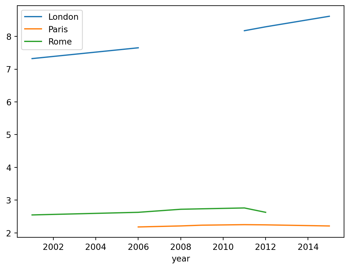
If you have a variable containing a DataFrame (like we do with census), you can plot it as a line graph using:

census.plot()

From this we can quickly see the missing data showing as gaps in the graph, and also that there are no clearly anomalous entries.

If you want to dive deeper into how this graph can be improved visually, you can see a short aside which covers that, but which does use some tools that we will not cover until later chapters.

Exercise

Read the file meantemp_monthly_totals.txt into Pandas. This data is originally from the Met Office and there’s a description of the format there under “Format for monthly CET series data”. It contains some historical weather data for a location in the UK. Import that file as a Pandas DataFrame using read_csv(), making sure that you set the index column, skip the appropriate rows, separate the columns correctly and cover all the possible NaN values.

Hint: This data is a little tricky to deal with as it uses spaces to separate its columns. You can’t just use sep=" " as that will assume that a single space is the separator. Instead of using sep at all, you need to tell it to use whitespace (e.g. spaces, tabs, etc.) as the delimiter (search the documentation for an appropriate argument).

Answer

import pandas as pd

Firstly, if we read the data in without passing any extra arguments, we get:

temperature = pd.read_csv(
    "./data/meantemp_monthly_totals.txt",
)
temperature.head()

	Mean Central England Temperature (Degrees Celsius)
1659-1973 Manley (Q.J.R.METEOROL.SOC.	1974)
1974 on Parker et al. (INT.J.CLIM.	1992)
Parker and Horton (INT.J.CLIM.	2005)
Year Jan Feb Mar Apr May Jun Jul Aug Sep Oct Nov Dec Annual	NaN
1659 3.0 4.0 6.0 7.0 11.0 13.0 16.0 16.0 13.0 10.0 5.0 2.0 8.9	NaN

So we need to dot he same as before, setting the skiprows argument:

temperature = pd.read_csv(
    "./data/meantemp_monthly_totals.txt",
    skiprows=4,  # skip first 4 rows of the header
)
temperature.head()

	Year Jan Feb Mar Apr May Jun Jul Aug Sep Oct Nov Dec Annual
0	1659 3.0 4.0 6.0 7.0 11.0 13...
1	1660 0.0 4.0 6.0 9.0 11.0 14...
2	1661 5.0 5.0 6.0 8.0 11.0 14...
3	1662 5.0 6.0 6.0 8.0 11.0 15...
4	1663 1.0 1.0 5.0 7.0 10.0 14...

It’s not separating the columns correctly so if we look at the data and see spaces, we might think that useing sep=" " would work, but if we try it:

temperature = pd.read_csv(
    "./data/meantemp_monthly_totals.txt",
    skiprows=4,
    sep=" ",  # try this...
)
temperature.head()

	Unnamed: 0	Unnamed: 1	Year	Unnamed: 3	Unnamed: 4	Unnamed: 5	Jan	Unnamed: 7	Unnamed: 8	Unnamed: 9	...	Unnamed: 43	Unnamed: 44	Unnamed: 45	Nov	Unnamed: 47	Unnamed: 48	Unnamed: 49	Dec	Unnamed: 51	Annual
0	NaN	NaN	1659	NaN	NaN	NaN	3.0	NaN	NaN	NaN	...	NaN	2.0	NaN	NaN	NaN	8.9	NaN	NaN	NaN	NaN
1	NaN	NaN	1660	NaN	NaN	NaN	0.0	NaN	NaN	NaN	...	NaN	5.0	NaN	NaN	NaN	9.1	NaN	NaN	NaN	NaN
2	NaN	NaN	1661	NaN	NaN	NaN	5.0	NaN	NaN	NaN	...	NaN	6.0	NaN	NaN	NaN	9.8	NaN	NaN	NaN	NaN
3	NaN	NaN	1662	NaN	NaN	NaN	5.0	NaN	NaN	NaN	...	NaN	3.0	NaN	NaN	NaN	9.5	NaN	NaN	NaN	NaN
4	NaN	NaN	1663	NaN	NaN	NaN	1.0	NaN	NaN	NaN	...	NaN	5.0	NaN	NaN	NaN	8.6	NaN	NaN	NaN	NaN

5 rows × 53 columns

That doesn’t look right. This is because sep=" " means “use a single space” as the separator, but in the data most columns are separated by multiple spaces. To make it use “any number of spaces” as the separator, you can instead set sep=r'\s+':

temperature = pd.read_csv(
    "./data/meantemp_monthly_totals.txt",
    skiprows=4,
    sep=r'\s+',  # whitespace-separated columns
)
temperature.head()

	Year	Jan	Feb	Mar	Apr	May	Jun	Jul	Aug	Sep	Oct	Nov	Dec	Annual
0	1659	3.0	4.0	6.0	7.0	11.0	13.0	16.0	16.0	13.0	10.0	5.0	2.0	8.9
1	1660	0.0	4.0	6.0	9.0	11.0	14.0	15.0	16.0	13.0	10.0	6.0	5.0	9.1
2	1661	5.0	5.0	6.0	8.0	11.0	14.0	15.0	15.0	13.0	11.0	8.0	6.0	9.8
3	1662	5.0	6.0	6.0	8.0	11.0	15.0	15.0	15.0	13.0	11.0	6.0	3.0	9.5
4	1663	1.0	1.0	5.0	7.0	10.0	14.0	15.0	15.0	13.0	10.0	7.0	5.0	8.6

That looks much better! Now we set the index_col:

temperature = pd.read_csv(
    "./data/meantemp_monthly_totals.txt",
    skiprows=4,
    sep=r'\s+',
    index_col="Year",  # Set the index
)
temperature.head()

	Jan	Feb	Mar	Apr	May	Jun	Jul	Aug	Sep	Oct	Nov	Dec	Annual
Year
1659	3.0	4.0	6.0	7.0	11.0	13.0	16.0	16.0	13.0	10.0	5.0	2.0	8.9
1660	0.0	4.0	6.0	9.0	11.0	14.0	15.0	16.0	13.0	10.0	6.0	5.0	9.1
1661	5.0	5.0	6.0	8.0	11.0	14.0	15.0	15.0	13.0	11.0	8.0	6.0	9.8
1662	5.0	6.0	6.0	8.0	11.0	15.0	15.0	15.0	13.0	11.0	6.0	3.0	9.5
1663	1.0	1.0	5.0	7.0	10.0	14.0	15.0	15.0	13.0	10.0	7.0	5.0	8.6

And, as we should always do, we plot the data we’ve just read in:

temperature.plot()

Something is wrong with this. There’s a line on the right-hand side which seems wrong. If we look at the last few lines of the data to see what’s going on:

temperature.tail()

	Jan	Feb	Mar	Apr	May	Jun	Jul	Aug	Sep	Oct	Nov	Dec	Annual
Year
2018	5.3	3.1	5.0	9.9	13.3	16.1	19.3	16.8	13.7	10.5	8.3	6.8	10.7
2019	4.0	6.9	7.9	9.1	11.2	14.2	17.6	17.2	14.3	9.8	6.2	5.7	10.4
2020	6.4	6.4	6.8	10.5	12.6	15.3	15.8	17.7	14.0	10.4	8.5	4.9	10.8
2021	3.2	5.3	7.3	6.5	10.3	15.5	17.8	16.0	16.0	12.0	7.2	6.3	10.3
2022	4.7	6.9	8.0	9.2	13.1	14.9	-99.9	-99.9	-99.9	-99.9	-99.9	-99.9	-99.9

We can see there are some -99.9 in the data, repsenting missing data. We should fix this with na_values:

temperature = pd.read_csv(
    "./data/meantemp_monthly_totals.txt",
    skiprows=4,
    sep=r'\s+',
    index_col="Year",
    na_values=["-99.9"]
)
temperature.tail()

	Jan	Feb	Mar	Apr	May	Jun	Jul	Aug	Sep	Oct	Nov	Dec	Annual
Year
2018	5.3	3.1	5.0	9.9	13.3	16.1	19.3	16.8	13.7	10.5	8.3	6.8	10.7
2019	4.0	6.9	7.9	9.1	11.2	14.2	17.6	17.2	14.3	9.8	6.2	5.7	10.4
2020	6.4	6.4	6.8	10.5	12.6	15.3	15.8	17.7	14.0	10.4	8.5	4.9	10.8
2021	3.2	5.3	7.3	6.5	10.3	15.5	17.8	16.0	16.0	12.0	7.2	6.3	10.3
2022	4.7	6.9	8.0	9.2	13.1	14.9	NaN	NaN	NaN	NaN	NaN	NaN	NaN

temperature.plot()